

How to draw a Decision Tree in R
This article has been written in continuation of one of the previous articles covering :1. What is Entropy ?
2. What is Information Gain?
We had explored how Decision Tree assigns variables on the basis of Information Gain. Now we will learn how to draw a decision tree in R on a telecom industry example and would understand the behind scene algorithm once again.
Ready ... Steady ... Go !
Download the data using following link, save it in your PC and note down the location.
Decision Tree in R :
A Decision Tree can be generated using rpart package in R. The structure of he code is :
rpart(formula, data=, method=,control=)
| formula | dependent ~ independent1+independent2+etc. |
| data= | data frame |
| method= | "class" for a classification tree |
| control= | optional parameters for controlling tree growth. For example, control=rpart.control(minsplit=30, cp=0.001) requires that the minimum number of observations in a node be 30 before attempting a split and that a split must decrease the overall lack of fit by a factor of 0.001 (cost complexity factor) before being attempted. |
# First you need to install the package in R
install.packages("rpart") # Installs packages rpart
library(rpart) # Loads rpart library
data1<-read.csv("C:\\Users\\data for decision tree in R.csv")
# Importing data, you need to customize the code with your file's location
# Fit tree
tree<-rpart(Leave.service~ Bill+Gender+std,method="class",data=data1,
control=rpart.control(minsplit=0, cp=0.001))
# Plot tree
plot(tree, uniform=TRUE, main="Classification Tree for Telecom")
text(tree, use.n=TRUE, all=TRUE, cex=.6)

So we have got the decision tree, now let's see how to interpret the same and also understand how R or any other software draw decision tree, using Entropy and Information gain base algorithm.
If Entropy and Information gain terms look alien to you, please go through our Previous blog in this series.
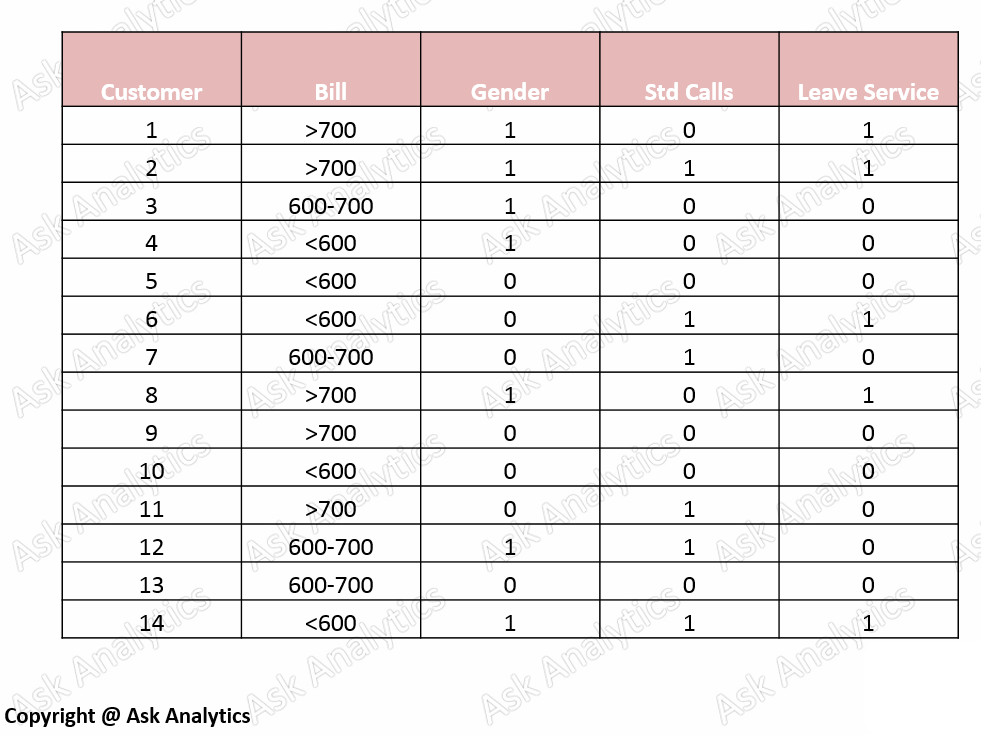
Our data looks like >>
There are four variables given in the data:
Monthly Billing : monthly bill of each individual
Gender : 1- Male , 0-female
Std : 1- taken std facility, 0 - has not taken std facility
Leave service : 1 - Customer has moved to other telecom operator, 0- continuing services with same operator
It first calculates the entropy of each variable for every bucket :
Entropy of Monthly Billing variable:

Entropy of Gender variable :


Then it calculates the information gain:

Since the monthly billing has maximum information gain value, it simply means that this variable has maximum ability to reduce the uncertainty and has best prediction ability.
So, monthly billing would be the root variable in decision tree.

Now we have to analyse only observations in which monthly billing is either >700 or <600.
We need to again calculate the information gain to further decide tree node.


We will continue this process at each node to reach to the best separation of 1 and 0.
The final tree after this process would be

I hope you have now crystal clear understanding of how decision tree works.
Enjoy reading our other articles and stay tuned with ...
Kindly do provide your feedback in the 'Comments' Section and share as much as possible.
D6A7A69151
ReplyDeletekiralık hacker
hacker arıyorum
belek
kadriye
serik
5382BFDAED
ReplyDeleteBeğeni Satın Al
EFT ile Takipçi
Tiktok Takipçi Arttırma